Precisely Forecasting Price Ranges with Volatility

Using a tool like Bollinger Bands® to forecast future price ranges is a time-honored technique but its calculations are simplified and in some situations flawed. Incorporating the log-normal nature of stock prices into the calculations gives better answers.

One greed-inducing aspect of volatility is that it enables us to make theoretically sound forecasts about the future.  It doesn’t matter whether it’s stock prices, annual rainfall, or deaths by shark attack, we can often use past volatility as a way of quantifying the probability of future values.  Volatility doesn’t enable us to predict whether average values are going to go up or down (sometimes we can use long-term averages for that) but it does allow us to make statistically valid predictions of the plus/minus ranges we can expect.  Of course, there are assumptions (e.g., that the level of volatility remains stable) but typically those are reasonable baselines.

Techniques like Bollinger Bands®, Probability Cones, and Z-scores use simplified calculations for computing price ranges.  For low levels of volatility and relatively short time periods their errors are small but as time and volatility increase your results can be significantly wrong or even nonsensical.  Given that institutional money is at stake, option pricing techniques such as the Black-Scholes equation and binomial tree calculations don’t take such shortcuts.

The incorrect assumption of the simplistic calculations is that since plus and minus returns are typically symmetrical, price ranges are symmetrical too.  As a simple counterexample, consider the end results for two symmetrical sequences of returns: three +2% days in a row, versus three -2% days in a row.  In the uptrend case, the final price increase factor would be (1+.02)³ = 1.0612, 6.12% higher than the starting price, and the downtrend price would be (1-.02)³ = 0.9412, 5.88% lower.  Not symmetrical!

Enter the Lognormal

As a result of this asymmetry, values of tangible things like stock prices, rainfall, and shark attacks that can’t go below zero often end up having what’s called a log-normal distribution.  These distributions are skewed to the right with a fatter right tail and a truncated left tail.

The chart below is a histogram showing the distribution of annual rainfall in Boulder Colorado for the last 123 years.

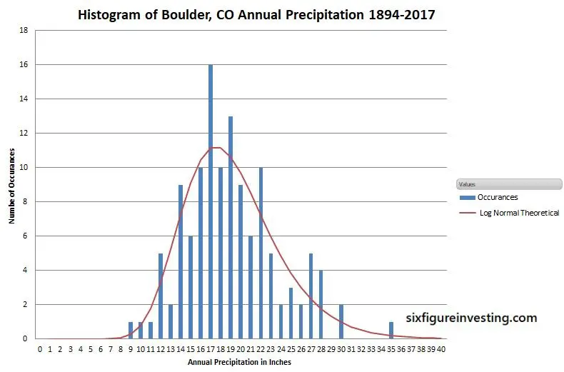
The horizontal axis has one-inch bins for annual rainfall (e.g., 12.3 and 12.8 would both go into the “12” bin) and the vertical axis is the number of occurrences of yearly rainfall that landed in that bin).

The red line calculation uses the volatility of annual rainfall along with log-normal statistics to predict Boulder’s annual rainfall distribution—not a bad match to the historical data.

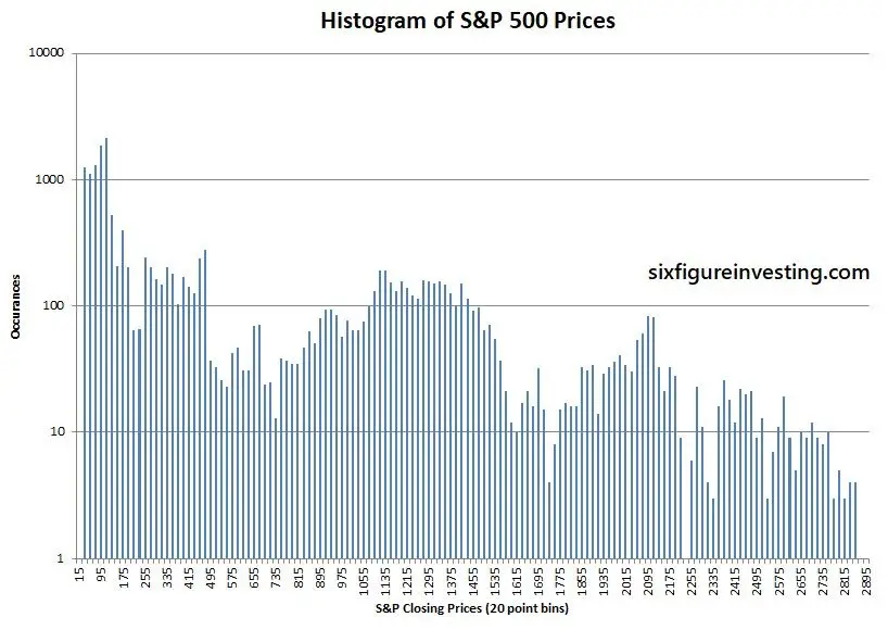
Historical price distributions of stock prices generally don’t have a log-normal shape because there’s another confounding factor—long-term growth.  The average annual rainfall in Boulder hasn’t changed much in the last 123 years but stock prices are usually different—the stocks that stick around tend to grow. Persistent growth smears out the price distributions over time.  Illustrating that, the chart below shows the simple histogram of S&P 500 prices since 1950—no log-normal in evidence.

We can remove the impact of growth by adjusting the price data with the time-series’ average growth rate—this is a calculation similar to using historic inflation rates to adjust for the buying power of a currency.

In the case of the S&P 500 the compounded growth since 1950 has been 0.0295% per day.  If we compound that value daily we obtain a factor that adjusts the price for the constant growth component of the S&P 500.  For example, the April 5^th, 2018 S&P index closed at 2662.84.  We can remove the cumulative average growth from that value by dividing it by the compounded average growth factor (1+0.000295)¹⁷¹⁷⁵ = 158.52, where the 17175 is the number of trading days since January 3^rd, 1950.  The adjusted price is thus $16.80.  Applying this adjustment technique to the entire S&P 500 daily time series we get the price distribution chart below:

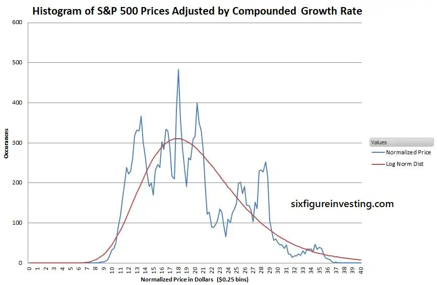
Not pretty—but recognizably log-normal.

When trying to predict future price ranges the analysis needs to take into account that stock prices are log-normally distributed—not Gaussian.

Transforming the Log-normal

Mathematically, dealing directly with log-normal distributions is ugly.  To simplify things the standard approach uses a mathematical transform.  A good transform converts a problem that’s tough to solve with default techniques into a different framework where the problem is easier to solve.  For example, it’s tough to physically copy a shirt directly (absent a suitable 3-D printer) but if the shirt is transformed—taken apart at the seams, the resulting pieces of cloth can be used to make a two-dimensional pattern.  With a pattern, it’s easy to make copies.  In the case of log-normal distributions, the logarithm function or “log” for short is the transformational equivalent of seam ripping.

If you take the log (usually base e, known as the natural logarithm LN) of each data point in a price history, you transform the distribution from a log-normal one into a normal one—we are now in “Log World”.  Standard statistical tools can now be used with this normal distribution.

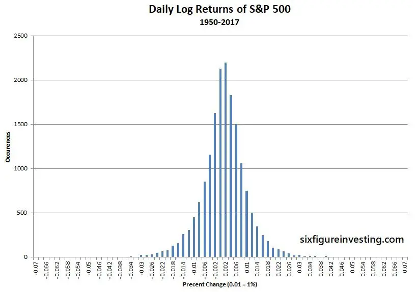
However, this first step doesn’t solve the problem of growth smearing the data—we resolve that by utilizing the period to period differences (returns) rather than the log prices. You can write this step as ln(P_n) – ln(P_n-1), where n equals the period number. Mathematically these log and return calculations can be combined into one compact operation: ln (P_n /P_n-1). This formula is often called the “log-returns” calculation.  When we convert stock price histories into log-returns we get nice symmetric distributions suitable for forecasting.  The chart below shows the log-returns distribution for the S&P 500.

Now, in preparation for doing our price projections, we can compute the statistical average growth rate (mean) and the volatility of this distribution using standard tools applicable to Gaussian distributions.  The average of the log returns is the geometric mean (the continuously compounded version), which I’ll call GM_CC. The volatility of the returns is computed by taking the sample standard deviation of the log returns.  Be aware that both of these numbers were computed in Log World so they don’t directly relate to prices.  Also, be aware that volatility is usually quoted in annualized terms—which enables apples-to-apples comparisons between different securities or time period lengths.  However for the calculations that follow we must keep the time period of the mean and standard deviation the same as the data set being used (typically daily).

Projecting Some Prices—the Median Forecast

Now that we have the key parameters we can move on to predicting some prices.

The simplest prediction is the median price.  Statistically 50% of the time the actual closing price will be higher than the forecasted median price and 50% of the time the actual price will be lower.  The formula for the forecasted median price is:

P_n = P_s* e^(GMcc*n)

Where:

• P_n = median price n periods in the future
• P_s = starting price
• e = Euler’s number ( approximately 2.71828) , in Excel use the EXP() function
• GM_cc = Geometric Mean (continuously compounded version)
• n = desired number of trading periods in the future for the forecast

So, for example, using historic parameters for the S&P 500, if the S&P is at 2900 and you want to estimate the median price point 21 trading days in the future the answer would be:

P_{21 =}   2900 * e^{(.000295*21)   =}  2918     (+0.62%)

The “e” in the “e^(GMcc*n) “ part of the equation converts things from “Log World” back to log-normally distributed prices.  It’s the equivalent of what a sewing machine does in my clothing analogy—transforming pieces of cloth back into real-world clothing.

The key assumptions are that the log-returns are normally distributed and that the geometric mean stays stable.  If the average growth rate of the stock starts trending up or down then all bets are off.

The trading period can be any consistent period of time—days, minutes, months, etc.  The only restriction is that the geometric mean and standard deviation need to be computed using data with the same period length.

Enter Volatility

For a median price estimate, we only need the geometric mean but traders and investors are often interested in probabilities other than 50-50.  To make those estimates, we also need to know the estimated volatility of the underlying security.  The volatility is a key component because it quantifies how widely a price is likely to diverge from its current price —for example, the odds of a low volatility utility stock increasing 10% in the next month might be quite low but a volatile tech stock might easily move that much or more.

The probabilities associated with volatility have a fixed relationship to the standard deviation.  For example, if returns are normally distributed the probability of a stock’s one-day percentage up move exceeding one standard deviation (+1 sigma) is ~16% and the odds of it exceeding a two standard deviation move (+2 sigma) is ~2.23%.  The generalized equation, which adds a volatility term, predicts upside price points over time:

P_n = P_s * e^{(GMcc*n+k*stdev*square root (n))}

Where:

• stdev = sample standard deviation of the log returns (in Excel: STDEV.S())
• k = multiplication factor, where 1 = 1 sigma, 2 = 2 sigma

Yes, that square root of the number of periods in the added volatility term is weird.  See Volatility and the Square Root of Time for more on that topic

For the sake of convenience, we usually use integer values of k but if you need different probabilities (e.g., quartiles) it’s straightforward to compute them.  For example, if you need to know the price that will not be exceeded 75% of the time k is +0.67, for 90% the k factor is +1.28.

If we want to want to compute a S&P index value that should statistically only be exceeded 16% of the time, (+1 standard deviation or one sigma) 21 days from now, we can compute:

P_21+16%  = 2900 * e^{(0.000295*21 + 1* 0.01*square root (21))}    =   3054.85    (+5.34%)

If we want to compute the upside S&P price 21 days from now, that only has a 2.23% chance (+2 sigma) of being breached, we compute:

 P_21+2.5%  = 2900 * e^{(.000295*21 + 2* 0.01*square root (21))}    =  3198.10    (+10.28%)

The Downside—Similar but not Symmetrical

The downside equation is similar but instead of adding the volatility term we subtract it.

P_n = P_s * e^{(GMcc*N – k* stdev*square root (n))}

If we want to want to compute a downside S&P index value that should statistically only be breached 16% of the time (-1 standard deviation or minus one sigma) 21 days from now we compute:

P_21-16%  = 2900 * e^{(0.000295*21 – 1* 0.01*square root (21))}    =  2787.3   (-3.89%)

Because of the log-normal nature of stock prices, the downside percentage for a -1 sigma move is less than the 1 sigma upside move.

The key assumptions for these equations are the same as the median prediction with the additional restriction that the volatility of the stock stays consistent.  If volatility really picks up or fades then all bets are off.

Making Things Simpler—but Sometimes Too Simple

Popular and useful tools like Bollinger Bands®, Probability Cones, and Z-scores use a simpler approach.  Usually, they assume the median price forward is today’s price and leave out the exponential function. Their approach to projecting price ranges is to increase it from the starting price by +k*stdev* square root(n) and decrease by –k*stdev* square root (n).  These simpler formulas are reasonable if durations are short (e.g., 2 months or less) and volatilities, as well as sigma levels, are low.  For the S&P 500, the typical error on the median price for 21 trading days would be around -0.5%, and the 1 sigma price bands errors will be around 2.2%.

On the other hand, if you are using higher sigma levels (e.g., Bollinger Bands default to 2), longer periods of time, larger geometric means, and/or securities with high volatilities (e.g., TSLA, NFLX, VXX, UVIX, SVIX, UVXY) then the errors become significant. For example, the 2X leveraged volatility fund, Volatility Shares’ UVIX—typically has a large geometric mean (e.g., -0.5%), and a high standard deviation (e.g., 4%).  With those characteristics, the error using the simplified calculation after 21 days on the median is -5%, the one sigma high/low band errors are -3% and 15%, and the 2 sigma high/low ranges have errors of -12% and +25%.

Monte Carlo Simulation Validation

As a cross-check of this analysis, I ran a Monte Carlo simulation of a test stock similar to Google (GOOG) with a daily geometric mean (.07%) and standard deviation (2%).  The simulation models the “random walk” behavior of a stock with the specified characteristics.

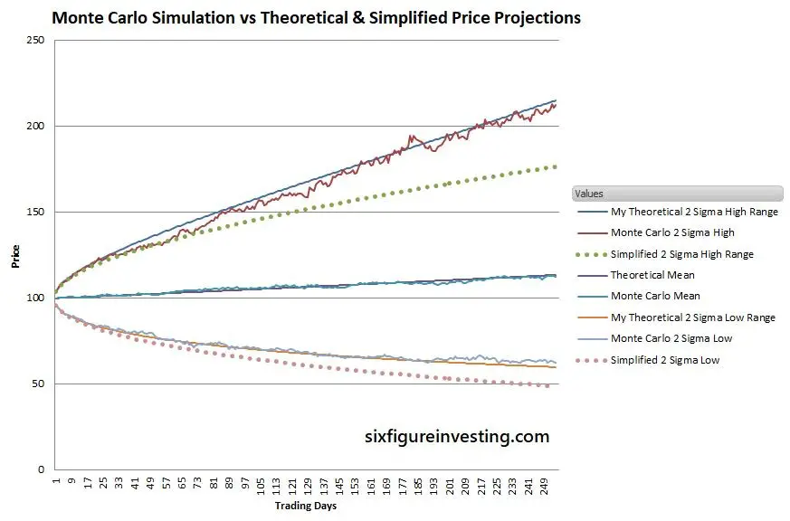
The smooth solid lines for high and low ranges are my two sigma theoretical projections.  The Monte Carlo lines show the first high and low simulated prices that are at the two sigma probability ranges (2.23%) for each period.  The dotted lines are the simplified estimates for high and low ranges using a Bollinger Band style analysis.

As you can see, the simplified analysis significantly underestimates the statistically expected ranges—after a year the predicted high range is 33% low and the low range is 28% low.

Conclusion

When the accuracy impact is low, it’s reasonable to simplify calculations to make them less intimidating or reduce the computational burden but it’s important to understand when those simplifications aren’t appropriate.  When habitually using these oversimplifications not only do all the results become suspect, it also hinders our understanding of what’s really going on.

For anyone looking into the finer points of volatility-based price forecasts the equations incorporating the log-normal distribution of prices should be used.  Don’t create unnecessary distortions in your crystal ball.